Private AI Sizing: Users, Agents, Rooms, Cost per Token
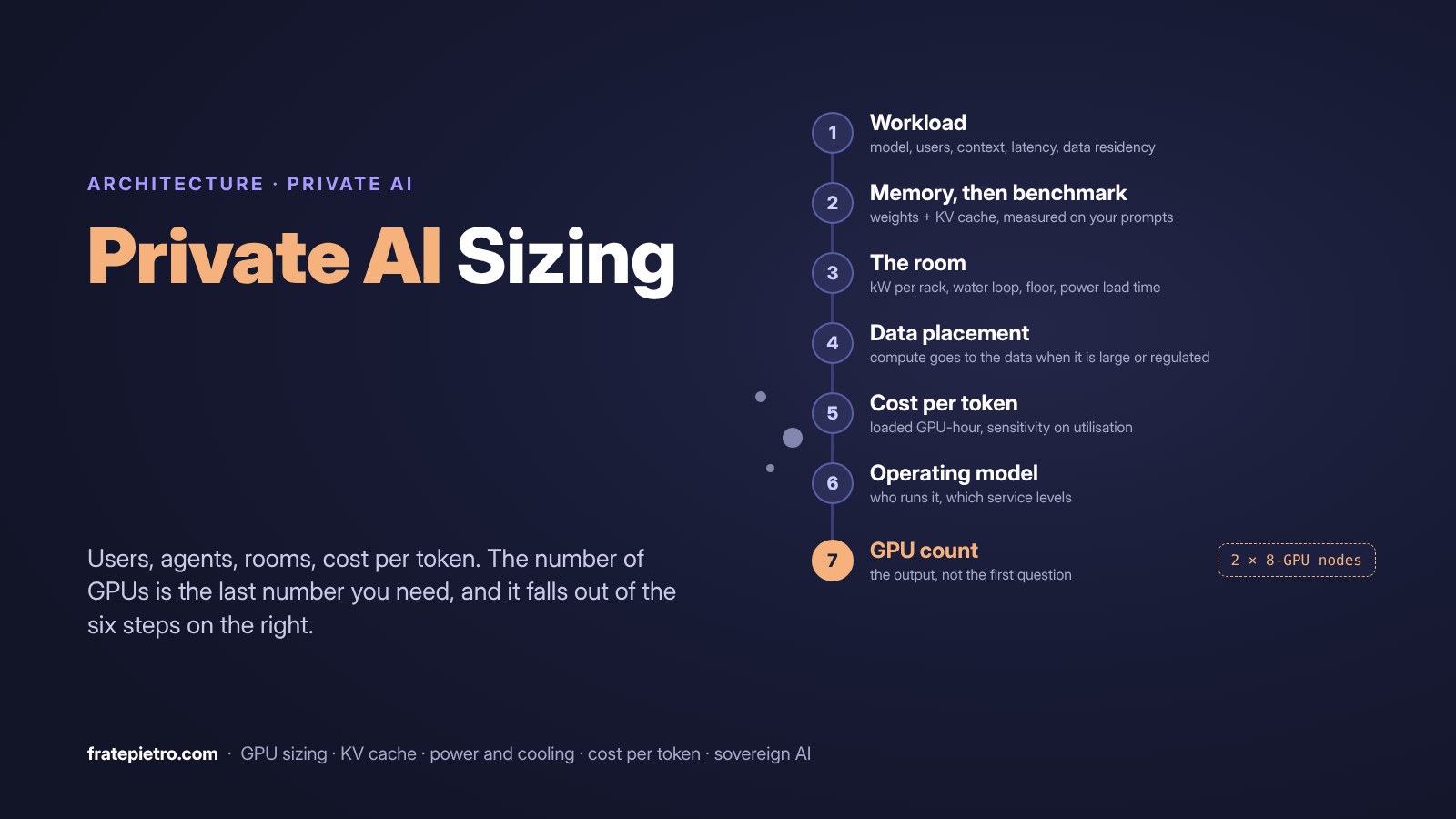
The conversation about private AI starts the same way almost every time. A team has a few use cases running on cloud GPUs, the bill is growing, and the business wants a predictable cost and control over where the data goes. The first question on the table is how many GPUs to buy.
I think this is the wrong first question. The number matters, and it is an output. Start from the GPU count and you get a quote. Start from the workload and you get a design, a cost you are able to defend, and a platform someone will run.
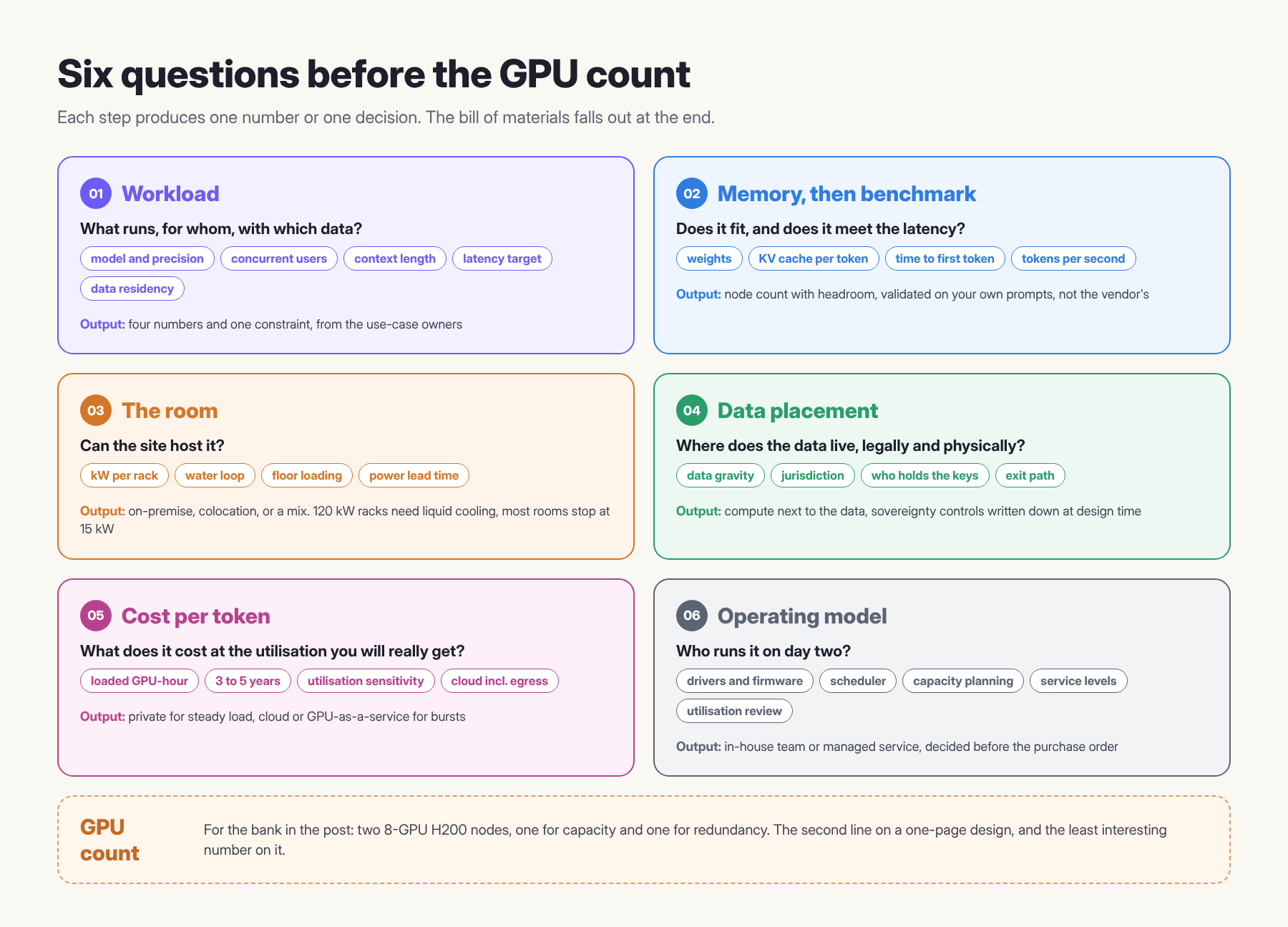
Most sizing guides skip the two steps where the uncertainty lives: how many requests are in flight at once, and what the regulator forces on the design. This post covers both with a bank as the running example, then memory, the room, data placement, cost, energy and operations. Prices and power figures are market observations from October 2026 and will age within months. GPU rental rates fell by a third in the past year alone. The formulas and the breakeven logic do not age. Keep the method, replace the inputs.
1. Write down the workload before you talk to a vendor
Four numbers decide most of the design, and they come from the people who own the use case: which model at which precision (a 70 billion parameter model in 8-bit is about 70 GB of weights, double that in 16-bit), how many requests are in flight at peak (not registered users, not daily users, requests being served right now), how long prompts and answers are (retrieval makes prompts long, and long prompts eat memory), and which latency the users will accept. Add one constraint: where the data is allowed to live. For the bank, in the country, on hardware the bank controls.
Then name the profile. Peter Ableda’s sizing guide for private AI sorts workloads into four: the chatbot, where latency rules, the researcher with long prompts over documents, where the key-value cache rules, the agent, where hidden reasoning tokens produce spikes, and the processor, overnight batch, where only tokens per hour count. Each wants different hardware, and most platforms carry two or three.
One asymmetry sits under all four. Reading a prompt (prefill) is parallel and cheap. Writing the answer (decode) is one token at a time and expensive, because every token moves the whole model through memory. A 10-page summary and a 10-page story have similar token counts, and the summary finishes about a hundred times faster. So the input-to-output ratio belongs in the workload sheet. The bank’s assistant, 1,500 tokens in and 300 out, is cheap per request. An agent that drafts long notes is not.
From employees to requests in flight
The second number is the one nobody has. Sponsors know how many employees will get the assistant. The platform needs to know how many requests are being served at the same second. Little’s law from queueing theory crosses the gap: requests in flight = arrival rate x time per request.
Take a bank with 5,000 employees licensed for an internal assistant.
- Adoption. One consultancy’s copilot benchmarks put active users at 40 to 60 percent of licensed seats after six months, daily actives at 30 to 40 percent of monthly, slower in finance and healthcare. Call it 2,500 monthly and 1,000 daily users.
- Frequency. Three to five prompts a session, one or two sessions a day. Call it 6 prompts per daily user: 6,000 requests a day.
- Peak hour. Office traffic concentrates. Say 20 percent lands in the busiest hour: 1,200 requests, one every three seconds.
- Duration. A 1,500-token prompt and a 300-token answer at 30 tokens per second take about 10 seconds.
Little’s law: 0.33 requests per second x 10 seconds = 3 or 4 requests in flight at peak. With a safety factor of three for lumpy arrivals and launches, plan for 10 to 12. For 5,000 employees. One 8-GPU node serves this with most of its capacity idle.
“200 concurrent users” on a vendor slide means 200 requests in flight, which by this arithmetic is a bank with 50,000 to 100,000 daily users or a customer-facing assistant. Microsoft’s provisioned throughput sizing asks for the same inputs, peak requests per minute, prompt size, response size and cache rate, and its worked example of 1,000 requests per minute is consumer scale.
Vendor sizing often uses a busy ratio instead: one in four licensed users active at once, so 80 paralegals become 20 concurrent users. That counts open sessions, people reading and typing, not requests being served, and for chat the model is busy only a few percent of a session. The busy ratio sizes the sessions your gateway holds. Little’s law sizes the requests your GPUs serve. Confusing the two is how a 5,000-employee assistant gets 1,250 concurrent requests and four nodes it never uses.
Write the chain down: licensed, monthly active, daily active, prompts per day, peak hour share, seconds per request, requests in flight. Every link is an assumption the business owns and a number you will measure after launch.
Agents change every number in the chain
An agent is a loop: read, call a tool, read the result, plan again, repeat until done. Three things change.
Tokens per task. A chat exchange is a few hundred to a couple of thousand tokens. A five-step agent task in a fraud-check example runs to about 13,500 tokens, and analyst estimates for enterprise agents sit in a 5 to 30 times range over chat. At the far end, a Stanford and Michigan study of coding agents on SWE-bench found roughly a thousand times more tokens than a code chat, with input tokens and cache reads driving most of the cost and token use between runs of the same task varying up to 30 times.
Duration. A chat request lasts ten seconds, an agent run minutes, so the same tasks per hour produce many more runs in flight, each holding a growing context. And each run re-sends most of that context on every call, so prefix caching and cache-aware routing stop being optional.
Back to the bank. Give 200 operations staff an agent that checks a transaction against policy, pulls three documents and drafts a note: 20 runs a day each, 4,000 runs a day, 800 in the peak hour, each about 3 minutes and 15,000 tokens. Little’s law: 0.22 runs per second x 180 seconds = 40 runs in flight at 10 to 20 thousand tokens of context each, and 12 million tokens in the peak hour, or 3,300 tokens per second sustained. That is more load than the 5,000-employee assistant, from a group 25 times smaller.
The rule: size chat assistants from users and sessions, size agents from tasks per hour and tokens per task, and expect the agent line to dominate within a year.
Peaks, and what happens above them
Everything above is sized for the peak hour, and the peak hour is itself an average. Inside it, arrivals bunch: Monday at nine, the minutes after an all-hands email, an agent that fans out forty calls at once. A platform sized for 12 requests in flight will see 30 for a few seconds several times a day, and 100 once a quarter.
Agree two numbers with the business, not one: the peak you size for, which sets the GPU count, and the peak you refuse, which sets what the platform does above it. Above it there are three behaviours. Queue with a bound, so the user waits seconds instead of timing out. Shed with a retry signal, so clients back off instead of retrying into a full system. Or degrade: a smaller model, a shorter context, a lower priority for batch so the adviser or the clinician keeps their latency. Which applies to which workload is a business decision, and in a regulated environment an audit question, because “what did the platform do under load” gets asked after an incident.
Routing picks the GPU. Admission control decides whether to take the request at all, from free cache memory, remaining compute and concurrency limits. I covered how the serving engines implement it, and why agents need a different approach, in Admission control for distributed LLM inference. For sizing: the GPU count buys the sized peak, admission control buys survival above it, and a platform with bounded queues and priority classes needs less headroom, which is money.
Three rules follow. Size for the peak hour, not the peak second, and let admission control absorb the difference. Give agents their own concurrency budget, because one runaway run can take the capacity of a hundred chat users. And count refused and queued requests from day one, the earliest signal that the agent line is outgrowing the plan.
2. Size the memory, then benchmark
Inference is a memory problem first. Each GPU holds the weights plus the key-value cache, the working memory of every conversation in flight, about 0.32 MB per token in 16-bit for a Llama-class 70B. One H100 with 4-bit weights fits about 28 requests at 4K context and almost none at 128K, which is why context length is in step 1.
KV cache per token = 2 x layers x KV heads x head dimension x bytes per value
For the bank’s two workloads together, 12 chat requests at 8K context and 40 agent runs at 16K, the cache is about 750,000 tokens, around 240 GB in 16-bit or 120 GB in 8-bit. Add 70 GB of weights. One 8-GPU H200 node has about 1.1 TB of high-bandwidth memory, so the bank fits in one node with room to grow, two with redundancy. Pair it with host memory at 1.5 to 2 times the GPU memory for loading and staging. If the bank later wants full fine-tuning of the 70B model, the arithmetic changes: weights, gradients and optimizer state take about 16 bytes per parameter, 1.1 TB, which is why full fine-tuning designs start around 32 GPUs while LoRA fits in one node. Keep 5 to 10 percent of memory free for the serving engine, or the first long prompt at peak produces a crash rather than a slow answer. Choose precision by the task: 8-bit costs under one percent of accuracy on a 70B model and halves the weights, 4-bit halves them again and suits general assistants, and legal or clinical analysis may justify 16-bit and the extra GPUs. Memory is rarely the constraint for an internal platform. Throughput at the agreed latency is.
So stop trusting the paper here. Run the bank’s model on the bank’s prompts on the target hardware, and measure time to first token and tokens per second against the latency from step 1. NVIDIA’s benchmarking guide gives the method: sweep concurrency, plot throughput against time to first token, pick the highest throughput that still meets the target (250 ms for chat in their example), and divide peak requests per second by requests per second per server. Vendor benchmarks tend to use shorter prompts than yours, and NVIDIA’s published NIM performance figures come from TensorRT-LLM, so an untuned open-source engine such as vLLM lands 20 to 30 percent lower.
The curve has a shape. At low concurrency every added user is free: the GPU was idle, throughput rises, nobody slows down. Then it saturates, requests queue, and time to first token jumps from under a second to several. In Ableda’s legal example, a 70B model in 8-bit on two H100s holds about 800 ms up to 50 concurrent requests and reaches 8 seconds at 100. The knee of that curve, measured on your prompts, is the real capacity of a replica, and step 1 exists to tell you how far below it your peak sits.
3. The industry decides more than the model does
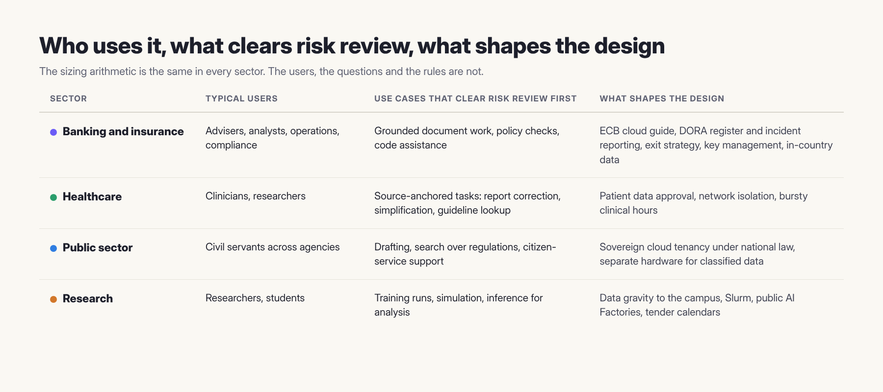
The arithmetic is the same in every sector. The users, the questions and the rules are not.
Banking shows the rules most clearly. In October 2026 Deutsche Bank deployed an AI platform inside its own environment so that client data and workflow activity stay inside the bank, and the reasons are written in the regulation. The ECB’s cloud outsourcing guide of July 2025, a benchmark in the 2026 supervisory cycle, expects data restricted to approved jurisdictions, an exit strategy with costs before go-live, concentration risk assessed across providers, disaster recovery tested yearly, and encryption with sound key management. Under DORA the platform is an ICT system in the register of information, incidents on it are reportable, and in November 2025 the supervisors put the three large hyperscalers under direct oversight as critical providers. A private or in-country deployment is the simplest answer to the data-location and exit questions, and open-weight models are an exit path in themselves.
Healthcare adds isolation before capacity. A German university hospital runs DeepSeek-R1 on-premise through vLLM behind network segmentation and egress filtering, with approval to process unanonymised patient data. Source-anchored tasks such as report correction scored well, open-ended conclusions produced clinical errors, and the platform is small in GPUs and large in security engineering. The public sector scales differently: “OpenAI for Germany” runs on SAP’s Delos Cloud, growing to 4,000 GPUs for millions of public employees, a sovereign-cloud tenancy under national law rather than hardware per ministry. Research institutions live in a batch scheduler, with data gravity to the campus and tender calendars longer than a hardware generation, which is why Helmholtz Munich moved about 300 servers to colocation and large training runs go to public AI Factories such as JUPITER.
4. Ask about the room before you ask about the rack
Power and cooling are not a detail. An H100 or H200 draws up to 700 W, a B200 1,000 to 1,200 W. An 8-GPU H100 node draws about 10 kW with server overhead, a B200 node 13 to 15 kW, and a GB200 NVL72 rack around 120 kW with liquid cooling to the chip. Most enterprise rooms were built for 5 to 15 kW per rack. Plan the feeds on datasheet maximums, not typical draw, with redundant supplies, and budget cooling at about 3,412 BTU per hour per kilowatt: four H100 servers are 41 kW and roughly 140,000 BTU per hour before switches and storage.
Four questions for the facility before anyone draws a rack:
- Kilowatts per rack, today and after the next upgrade of the room?
- A water loop, or a plan for one? Rear-door heat exchangers reach roughly 40 kW. Above that it is direct liquid cooling and coolant distribution units.
- Does the floor hold the weight?
- How long does extra power take to arrive? In some cities, years.
The bank’s room is built for 8 kW per rack. So on-premise means air-cooled nodes spread across racks, or the platform in an in-country colocation site with a dedicated line, or inference near the users and anything heavier in colocation. Three options, three prices, and the constraints pick one. The 120 kW rack was never on the list: a 70B model does not need 72 GPUs in one NVLink domain.
5. Decide where the data lives, then where the compute goes
Data accumulates. Every dataset, model and log lands in one place, and after a year or two moving any of it takes months: the egress fee is the small part, re-engineering pipelines and re-validating models the large one. So decide placement early and put compute next to the data when the data is large or regulated. For a research institute that means colocation with links to the campus. For the bank it means the same country and the same legal control, whatever the building.
Sovereignty follows, and it is more than a location: who can access data and models, including support staff and foreign law, who holds the keys, where hardware and support come from, and whether you are able to leave. Open-weight models help because you know what you are running. Write the controls down at design time. In banking the ECB guide is the list.
6. Cost per token, with real prices and the utilisation you will really get
The business case is the part engineers skip and the board reads. Everything comes from the loaded cost per GPU-hour:
cost per GPU-hour = (hardware amortised over 3 to 5 years + power + space + network + software + people) / (GPUs x hours x utilisation)
Fill it in with today’s numbers. In October 2026 an 8-GPU H100 system cost 250,000 to 320,000 dollars new, H200 and B200 systems quote-based above that. Electricity at 0.12 dollars per kWh and PUE 1.4 came to about 150 dollars per GPU per month, roughly 0.21 dollars per GPU-hour, about double at European industrial rates. Add 7,500 dollars a year of hosting and software per server, NVIDIA’s own example, and one platform engineer at 120,000 a year for two nodes, 0.86 dollars per GPU-hour on 16 GPUs.
At 100 percent utilisation that is about 2.20 dollars per GPU-hour in the US and 2.40 in Europe. Real utilisation is the divisor:
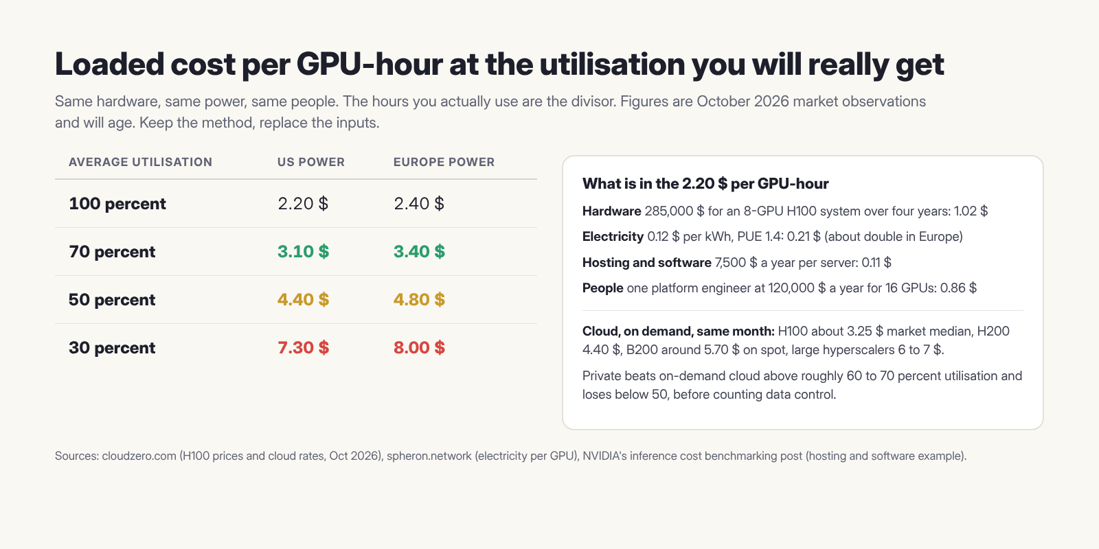
Compare with the cloud: the market median for an H100 was about 3.25 dollars per GPU-hour on demand, 4.40 for an H200, around 5.70 for a B200 on spot, and 6 to 7 at the large hyperscalers. At these prices a private platform beats on-demand cloud above roughly 60 to 70 percent utilisation and loses below 50, before counting data control. The crossover moves as both sides reprice, which is why the utilisation sensitivity, not the price, is the durable part of the case. One unit-economics analysis puts the breakeven against managed APIs above 8,000 conversations a day, which matches step 1.
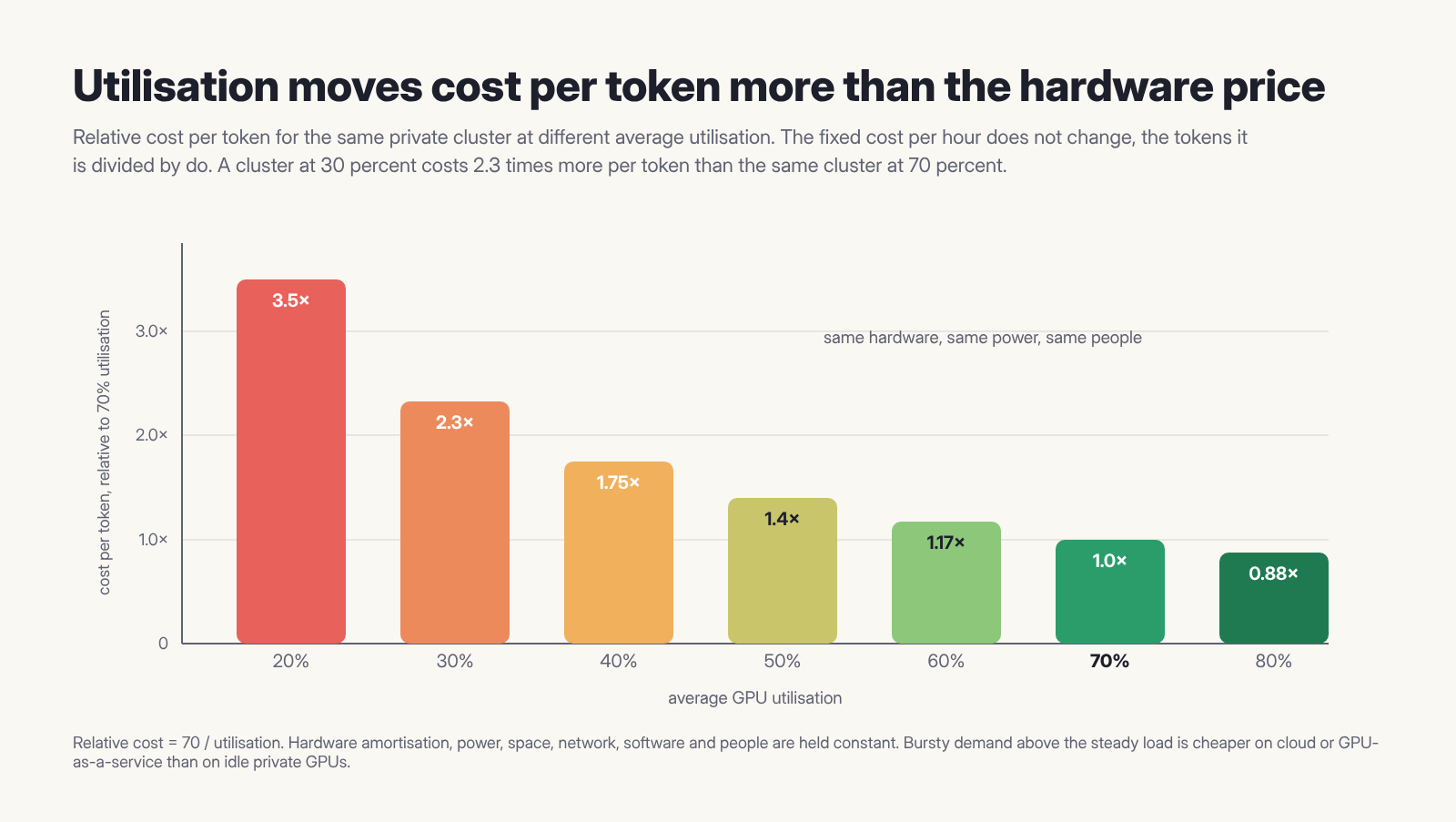
Now step 1 bites. The 5,000-employee assistant alone would run a node at a few percent utilisation outside the peak hour. The private case closes only when the platform carries steady work: the agent line, batch at night, several use cases on shared capacity. Chat assistants justify a cloud subscription. Agents, batch and regulated data justify a platform. The board comparison is three to five years of cost, cloud against private, with the utilisation sensitivity, egress and commitments on the cloud side and people on the private side. In most cases the answer is a hybrid: private for the steady load, cloud or GPU-as-a-service for the bursts.
7. Energy per token
Cost per token is energy per token with a price attached. Three reference points. Google measured a median Gemini text prompt at 0.24 watt-hours, about 860 joules, with 0.14 Wh on the accelerator and the rest in host, idle capacity and facility overhead, and a 33 times reduction per prompt over twelve months, 23 times from model changes and 1.4 times from utilisation. Microsoft Research puts optimised frontier inference at a median 0.31 Wh per query, says public estimates overstate production energy by 4 to 20 times, and finds that long reasoning and agent queries raise energy per request by more than an order of magnitude. At the token level, a Carnegie Mellon measurement on H200 puts Llama 3.1 8B at about 1.4 joules per output token at batch 16 and 2K context, and 5 to 6 joules per token at batch 1, a four times gap from batching alone.
For the bank’s node the estimate is direct and depends on the node’s draw and your tariff, not on a vendor. A 10 kW node at PUE 1.3 draws 13 kW. At the agent peak of 3,300 tokens per second that is about 4 joules per token, 1.1 kWh per million tokens, roughly 0.25 dollars of electricity per million at European rates. At 30 percent utilisation the node draws most of that power anyway, so energy per token roughly triples. The levers, in order: a smaller or quantized model, prefix caching, batching, and only then the hardware generation.
The hardware is moving too. NVIDIA’s Rubin platform, shipping from partners in the second half of 2026, claims up to 10 times lower cost per token than Blackwell for mixture-of-experts models, and its co-packaged optics switches claim 5 times better power efficiency than pluggable transceivers. Treat both as upper bounds until you run your own prompts, and remember that a faster rack is a denser, liquid-cooled rack, so step 4 comes back before the gain arrives.
8. Design the operating model with the hardware
First the build-or-rent check, which OneSource’s gated build guide reduces to three signals: rented GPUs busy most hours of most days, regulated or contract-restricted data, and projects delayed by quotas or missing capacity. Two of three point to building. Fewer, rent six more months and measure. For the bank the second is certain and the first depends on the agent line.
On day two someone owns drivers and firmware, the scheduler, capacity planning, incidents, patching, and a monthly report on utilisation, cost and energy per token. Decide who before the purchase order, because the answer changes the design. Researchers in Slurm and enterprise teams in Kubernetes need different platforms, and many organisations need both. If nobody in-house will run it, a managed service is part of the architecture, with service levels in the same document as the bill of materials. In a bank the operating model also answers DORA: who reports an incident, within which deadline, with which evidence.
Two items sizing guides leave out belong here. Acceptance testing with pass criteria written before the hardware arrives: GPU diagnostics on every card, a 24 to 72 hour burn-in, RDMA tests between every server pair, NCCL collectives across all GPUs, storage at checkpoint size, one representative workload at full scale, and a failure drill. Record the baselines, because they are how you detect drift a year later. And the team: GPU, network, storage and platform engineers, security, and an on-call rotation, which means several people or a provider. The scarce role is the fabric engineer, one reason even owners of hardware buy the operations.
Further reading, and what it leaves out
The guides this post stands on: VMware’s sizing guidance for latency targets, the KV-cache walkthrough for per-model memory, the users-to-GPU method, NVIDIA’s cost per million tokens, Microsoft’s throughput sizing, Ableda’s blueprint for memory and saturation, VMware’s Private AI Sizing Guide, and OneSource’s gated build plan for facility, acceptance and operations. All of them start from concurrent users or requests per minute as a given. None gets there from a headcount, budgets agents as a separate line, says what happens above the sized peak, or puts the regulator and the energy line next to the hardware.
The bank on one page
Workload: 5,000 employees on a 70B assistant, 8-bit, about 12 requests in flight at peak, plus 200 operations staff on an agent, about 40 runs in flight at 16K context, 2 seconds to first token, data in country. Above the sized peak: bounded queue for chat, priority classes with agents and batch below interactive users, shed with a retry signal beyond that.
Compute: two 8-GPU H200 nodes, one for capacity and one for redundancy, validated on the bank’s prompts, headroom for the agent line to triple.
Network: NVLink inside the node, Ethernet between nodes, because inference replicas stay inside a node and the operations team already runs Ethernet.
Storage: an all-flash tier for model loading and cache offload. A parallel file system waits until fine-tuning starts.
Facility: the 8 kW room will not host the nodes in one rack, so in-country colocation with a dedicated line, or air-cooled nodes across racks. Priced both ways.
Regulation: register of information entry, exit strategy with costs, keys under the bank’s control, incident reporting path, all written before go-live.
Cost and energy: loaded cost per GPU-hour, cost and energy per token at 40, 60 and 80 percent utilisation, against the current cloud bill including egress.
Operations: who runs it, which service levels, a quarterly utilisation review, and a count of queued and refused requests in the monthly report.
Every line traces to a requirement or a measurement, and every price carries a date. The GPU count is in the second line, and it is the least interesting number on the page. When someone asks how many GPUs they need, the useful reply is a question: for what, for whom and how often, chat or agents, under which regulator, in which room, and who will run it.